Replicating survey data
Marko Lalovic
Last Updated: 2024-03-28
Source:vignettes/articles/replicating_survey_data.Rmd
replicating_survey_data.Rmd
library(responsesR) # load responsesR
library(psych) # for the bfi data set

# optionally, to recreate the plots:
library("GGally")
#> Loading required package: ggplot2
#>
#> Attaching package: 'ggplot2'
#> The following objects are masked from 'package:psych':
#>
#>     %+%, alpha
#> Registered S3 method overwritten by 'GGally':
#>   method from
#>   +.gg   ggplot2
library(gridExtra)
library(cowplot)
This article covers the topic of replicating survey data in order to create scale scores.
Survey data
We will use bfi dataset from package ‘psych’ (Revelle 2024). It is made up of 25 personality items, and some demographic attributes such as gender and education for 2800 subjects:
library(psych)
str(bfi)
#> 'data.frame':    2800 obs. of  28 variables:
#>  $ A1       : int  2 2 5 4 2 6 2 4 4 2 ...
#>  $ A2       : int  4 4 4 4 3 6 5 3 3 5 ...
#>  $ A3       : int  3 5 5 6 3 5 5 1 6 6 ...
#>  $ A4       : int  4 2 4 5 4 6 3 5 3 6 ...
#>  $ A5       : int  4 5 4 5 5 5 5 1 3 5 ...
#>  $ C1       : int  2 5 4 4 4 6 5 3 6 6 ...
#>  $ C2       : int  3 4 5 4 4 6 4 2 6 5 ...
#>  $ C3       : int  3 4 4 3 5 6 4 4 3 6 ...
#>  $ C4       : int  4 3 2 5 3 1 2 2 4 2 ...
#>  $ C5       : int  4 4 5 5 2 3 3 4 5 1 ...
#>  $ E1       : int  3 1 2 5 2 2 4 3 5 2 ...
#>  $ E2       : int  3 1 4 3 2 1 3 6 3 2 ...
#>  $ E3       : int  3 6 4 4 5 6 4 4 NA 4 ...
#>  $ E4       : int  4 4 4 4 4 5 5 2 4 5 ...
#>  $ E5       : int  4 3 5 4 5 6 5 1 3 5 ...
#>  $ N1       : int  3 3 4 2 2 3 1 6 5 5 ...
#>  $ N2       : int  4 3 5 5 3 5 2 3 5 5 ...
#>  $ N3       : int  2 3 4 2 4 2 2 2 2 5 ...
#>  $ N4       : int  2 5 2 4 4 2 1 6 3 2 ...
#>  $ N5       : int  3 5 3 1 3 3 1 4 3 4 ...
#>  $ O1       : int  3 4 4 3 3 4 5 3 6 5 ...
#>  $ O2       : int  6 2 2 3 3 3 2 2 6 1 ...
#>  $ O3       : int  3 4 5 4 4 5 5 4 6 5 ...
#>  $ O4       : int  4 3 5 3 3 6 6 5 6 5 ...
#>  $ O5       : int  3 3 2 5 3 1 1 3 1 2 ...
#>  $ gender   : int  1 2 2 2 1 2 1 1 1 2 ...
#>  $ education: int  NA NA NA NA NA 3 NA 2 1 NA ...
#>  $ age      : int  16 18 17 17 17 21 18 19 19 17 ...
The personality items are split into 5 categories: agreeableness A1-5, conscientiousness C1-5, extraversion E1-5, neuroticism N1-5 and openness O1-5. Each item was answered on a six point scale ranging from 1 (very inaccurate), to 6 (very accurate).
Let’s focus only on the first 5 items corresponding to agreeableness. To investigate the differences in agreeableness between men and women we will also use the gender attribute.
avars <- c("A1", "A2", "A3", "A4", "A5")
data <- bfi[, c(avars, "gender")]
mapdf <- data.frame(old = 1:2, new = c("Male", "Female")) # Males = 1, Females =2
data$gender <- mapdf$new[match(data$gender, mapdf$old)]
head(data)
#>       A1 A2 A3 A4 A5 gender
#> 61617  2  4  3  4  4   Male
#> 61618  2  4  5  2  5 Female
#> 61620  5  4  5  4  4 Female
#> 61621  4  4  6  5  5 Female
#> 61622  2  3  3  4  5   Male
#> 61623  6  6  5  6  5 Female
Examine the data for missing values:
apply(data, 2, function(x) sum(is.na(x))/length(x))
#>          A1          A2          A3          A4          A5      gender
#> 0.005714286 0.009642857 0.009285714 0.006785714 0.005714286 0.000000000
Impute the missing values.
Save the new data set as a csv file.
write.csv(data, "../../data/bfi_agreeableness_and_gender.csv", row.names=FALSE)Reproducing item responses
Check the size of the male and female samples.
table(data$gender)
#>
#> Female   Male
#>   1881    919
Separate the items into two groups according to their gender.
avars <- c("A1", "A2", "A3", "A4", "A5")

items_M <- data[data$gender == "Male", avars]
items_F <- data[data$gender == "Female", avars]
To reproduce the items, start by estimating the parameters of the latent variables, assuming they are normal and providing the number of possible response categories ‘K = 6’:
params_M <- estimate_parameters(data = items_M, K = 6)
params_F <- estimate_parameters(data = items_F, K = 6)
params_M
#>          items
#> estimates         A1         A2         A3         A4         A5
#>        mu -0.6618876  0.8649575  0.7645033  0.8412600  0.7734527
#>        sd  1.0967866  0.7925097  0.8540241  1.1957912  0.8910793
params_F
#>          items
#> estimates         A1         A2         A3         A4         A5
#>        mu -1.1272393  1.1838317  1.0758738  1.3342088  0.9543986
#>        sd  1.1582560  0.7762984  0.8187612  1.4088157  0.8493250
Then, generate new responses to the items using the estimated parameters and correlations:
set.seed(12345) # to ensure reproducible results

new_items_M <- get_responses(n = nrow(items_M),
                             mu = params_M["mu", ],
                             sd = params_M["sd", ],
                             K = 6,
                             R = cor(items_M))

new_items_F <- get_responses(n = nrow(items_F),
                             mu = params_F["mu", ],
                             sd = params_F["sd", ],
                             K = 6,
                             R = cor(items_F))
Let’s compare the results, by plotting the correlations matrix with bar charts on the diagonal:
corr_plot <- function(df, title="") {
  pairs <- ggpairs(df,
                   upper = list(continuous = wrap(ggally_cor, stars=F, size=2)),
                   diag = "blank", lower = "blank")

  dff <- data.frame(df)
  for(j in 1:ncol(df)) {
    dff[, j] <- as.factor(df[, j])
  }
  pairsf <- ggpairs(dff, upper="blank", lower="blank", title=title) +
    theme(axis.line=element_blank(),
          text = element_text(size = 8),
          plot.title = element_text(size=10),
          axis.text=element_blank(),
          axis.ticks=element_blank())
  for(i in 1:ncol(df)) {
    for(j in 1:ncol(df)) {
      if (j > i) {
        pairsf[i, j] <- pairs[i, j]
      }
    }
  }
  return(pairsf)
}
p1 <- corr_plot(items_M, "Agreeableness items for man")
p2 <- corr_plot(new_items_M, "Reproduced agreeableness items for man")

p3 <- corr_plot(items_F, "Agreeableness items for women")
p4 <- corr_plot(new_items_F, "Reproduced agreeableness items for women")
plot_grid(ggmatrix_gtable(p1), ggmatrix_gtable(p2),
          ggmatrix_gtable(p3), ggmatrix_gtable(p4),  ncol = 2)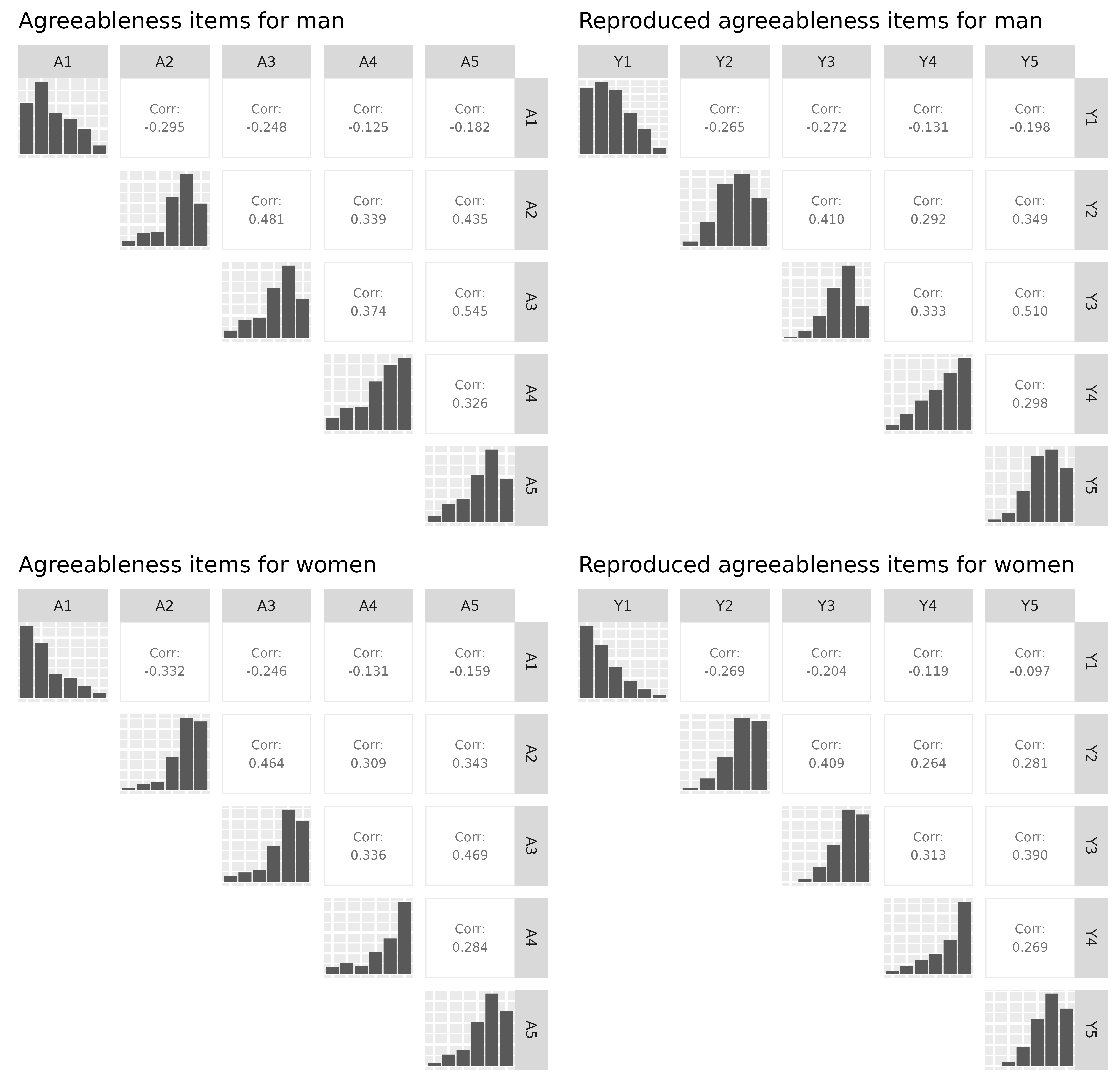
Recreating scale scores
The next step would be to create agreeableness scale scores for both groups of participants, by taking the average of these 5 items.
# Combine new items and gender in new_data data frame
new_data <- data.frame(rbind(new_items_M, new_items_F))
new_data$gender <- c(rep("Male", nrow(items_M)), rep("Female", nrow(items_F)))
head(new_data)
#>   Y1 Y2 Y3 Y4 Y5 gender
#> 1  3  5  5  4  5   Male
#> 2  1  5  4  4  4   Male
#> 3  2  6  5  6  4   Male
#> 4  4  4  4  6  5   Male
#> 5  4  5  3  2  2   Male
#> 6  5  4  5  6  5   Male

# We also need to reverse the first item because it has negative correlations
data$A1 <- (min(data$A1) + max(data$A1)) - data$A1
new_data$Y1 <- (min(new_data$Y1) + max(new_data$Y1)) - new_data$Y1

# Create agreeableness scale scores
data$agreeable <- rowMeans(data[, avars])
new_data$agreeable <- rowMeans(new_data[, c("Y1", "Y2", "Y3", "Y4", "Y5")])
And visualize the results with a grouped boxplot:
scale_boxplot <- function(data, title="") {
  xbreaks <- seq(from = 2, to = 6, length.out = 3)
  p <- ggplot(data, aes(x = agreeable, y = gender)) +
    geom_boxplot() +
    scale_x_continuous(breaks = xbreaks) +
    ggtitle(title) +
    theme(text = element_text(size = 8),
          plot.title = element_text(size=10),
          axis.title.y = element_blank())
  return(p)
}
p1 <- scale_boxplot(data, "Agreeableness in men and women")
p2 <- scale_boxplot(new_data, "Reproduced agreeableness in men and women")
plot_grid(p1, p2,  nrow = 2)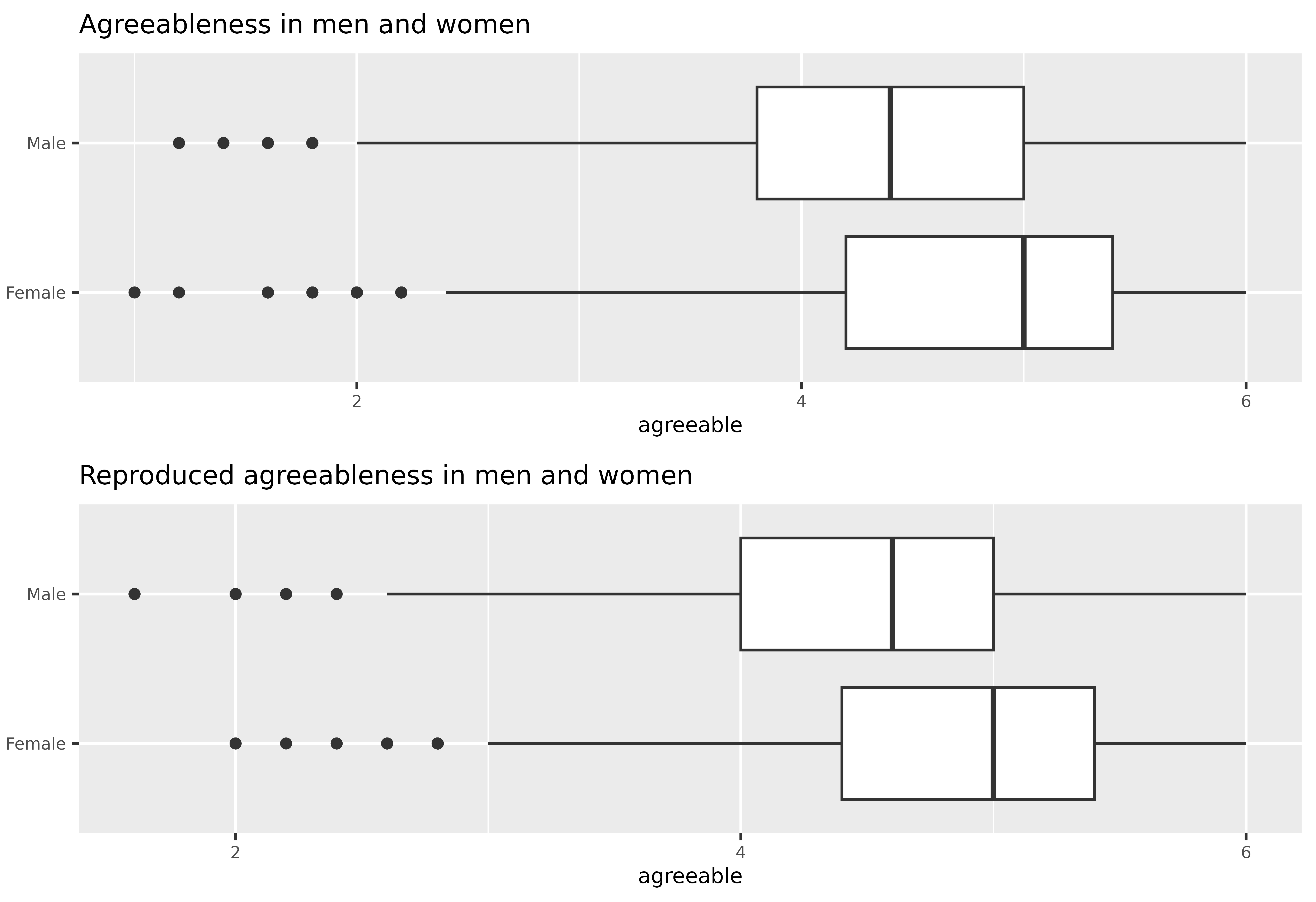
Finally, let’s also run Welch’s t-test to test if men and women differ on agreeableness using both data sets:
t.test(agreeable ~ gender, data = data)
#>
#>  Welch Two Sample t-test
#>
#> data:  agreeable by gender
#> t = 10.881, df = 1686.8, p-value < 2.2e-16
#> alternative hypothesis: true difference in means between group Female and group Male is not equal to 0
#> 95 percent confidence interval:
#>  0.3234122 0.4656518
#> sample estimates:
#> mean in group Female   mean in group Male
#>             4.782562             4.388030
t.test(agreeable ~ gender, data = new_data)
#>
#>  Welch Two Sample t-test
#>
#> data:  agreeable by gender
#> t = 12.616, df = 1648.4, p-value < 2.2e-16
#> alternative hypothesis: true difference in means between group Female and group Male is not equal to 0
#> 95 percent confidence interval:
#>  0.3281059 0.4489107
#> sample estimates:
#> mean in group Female   mean in group Male
#>             4.905157             4.516649