Topological features applied to the MNIST data set
Extraction of topological features that can be used as an input to standard algorithms to obtain qualitative geometric information.
Persistent homology is a fascinating mathematical tool that continues to be studied, developed, and applied. The purpose of this tutorial is to give a friendly introduction on how to use the persistent homology that does not require substantial knowledge of topological methods. To illustrate the use of persistent homology in machine learning we apply it to the MNIST data set of handwritten digits. A very similar approach can be applied to any point cloud data and can be generalized to higher dimensions.

The main problem we are trying to solve is how to extract the topological features that can be used as an input to standard machine learning algorithms. We will use a similar approach as described in [1].
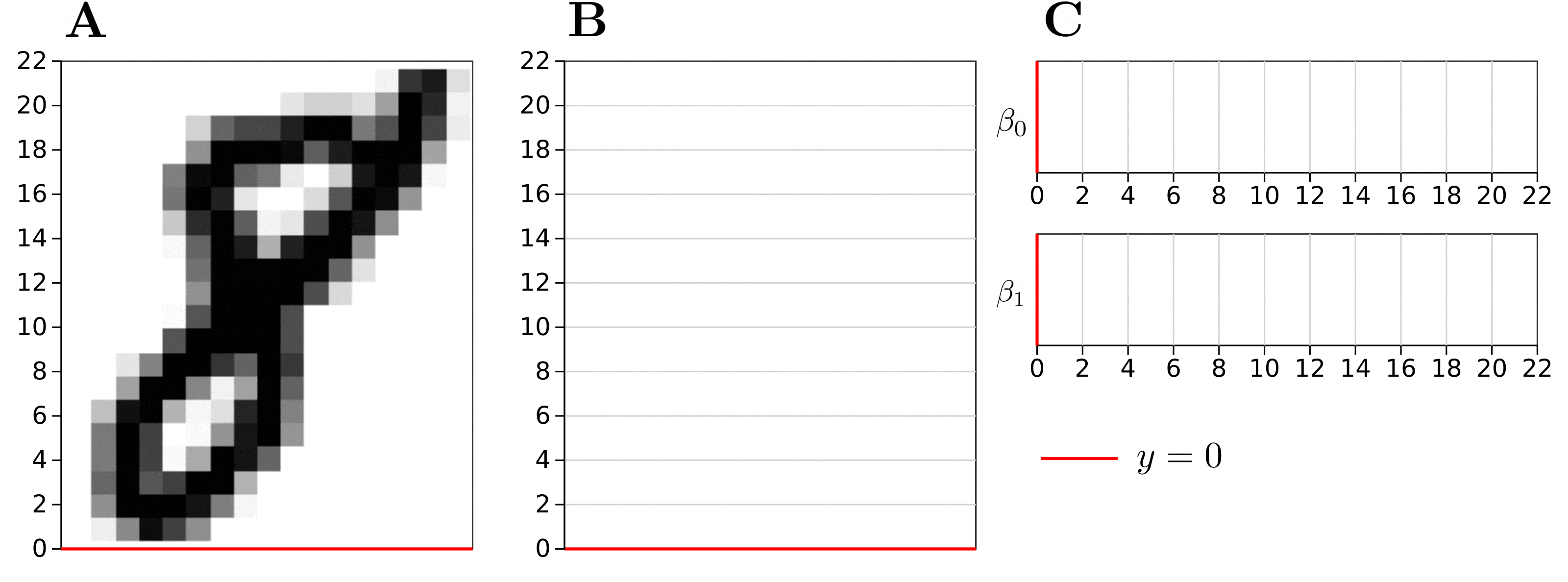
From each image, we first construct a graph, where pixels of the image correspond to vertices of the graph and we add edges between adjacent pixels; see Figure 1A and 1B. We then extract 0- and 1-dimensional topological features called Betti numbers denoted by $\beta_{0}$ and $\beta_{1}$. For example, a torus has one connected component so $\beta_{0} = 1$, and two cycles or loops so $\beta_{1} = 2$; see Figure 1C.
A pure topological classification cannot distinguish between individual numbers, as the numbers are topologically too similar. For example, numbers 6 and 9 are topologically the same if we use this style for writing numbers. Persistent homology, however, gives us more information.
(The pauses in the animation will be explained below, you can also play with this example interactively: here.)
We define a filtration on the vertices of the graph corresponding to the image pixels, adding vertices and edges as we sweep across the image in the vertical or horizontal direction; see Figure 2A and 2B. This adds spatial information to the topological features. For example, though 6 and 9 both have a single loop, it will appear at different locations in the filtration. We then compute the persistent homology given the simplex stream from the filtration to get the finite set of intervals called Betti barcodes; Figure 2C.
Finally, we extract 4 features from the k-dimensional barcode from the invariants discussed in [1]. For each of 4 sweep directions: top, bottom, right, left and dimensions: 0 and 1, we compute 4 features. This gives us a total of 32 features per image. On the extracted features from a set of images, we then apply a support vector machine (SVM) learning algorithm to classify the images.
Overview. First, we give some motivation and put the problem in a broader context of Topological Data Analysis and Computational Topology. Next, we explain the extraction of topological features on the simple example shown in Figure 2. Finally, we present and evaluate the empirical classification results on a subset of the MNIST database.
The aim is to demonstrate the classification potential of the technique and not to outperform the existing models. For a more interesting example of using this technique on a clinical data set to classify hepatic lesions, see [1].
I made publicly available all scripts including a processed version of the dataset. I am also using freely available computational topology package called Dionysus 2 for the computation of persistent homology.
Introduction
Topology applied to real-world data sets using persistent homology has begun to look for applications in machine learning, including deep learning [2]. Topology is mainly used in a pre-processing step to provide robust features for learning. Our data is often a finite set of noisy samples from some underlying space. The developed topological techniques, mostly deal with point clouds, i.e. finite sets of data points in space. Point clouds are typically captured by a variety of imaging devices, such as MRI or CT scanners. With the greater availability of such devices, this type of data is being generated at an increasing rate. The data sets are often also very noisy and contain a lot of missing information, especially biological data sets. Our ability to analyze this data, both in terms of the amount and the nature of the data, is clearly out of step with the data we generate [3]. Topology can be used to make a useful contribution to the analysis of such data sets and it is especially helpful in studying them qualitatively.
Terminology
- Topology is a branch of mathematics that deals with qualitative geometric information. This includes the classification of loops and higher-dimensional surfaces.
- Topological data analysis and computational topology deal with the study of topology using a computer.
- Persistent homology is an algebraic method for discerning topological features of data.
- Connected component (or connected cluster of points) is a 0-dimensional feature and cycle (or loop) is a 1-dimensional feature.
- Simplicial complex is a set composed of points, line segments, triangles, and their n-dimensional counterparts.
- Filtration is the sequence of simplicial complexes, with an inclusion map from each simplicial complex to the next.
- Barcode is a visual representation of the persistence of the topological features. Longer bars represent significant features of the data. Shorter bars are due to irregularities or noise.
Methods
Extracting the graph structure
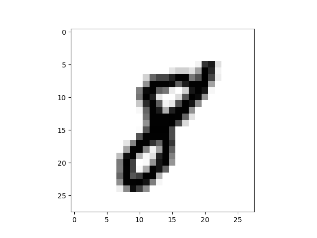
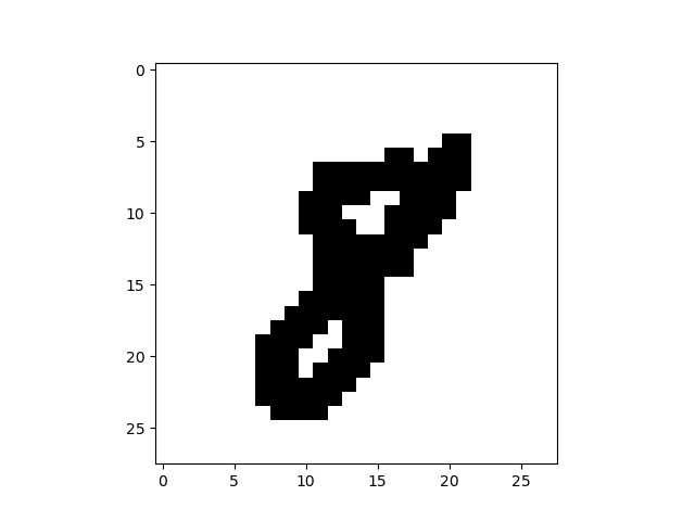
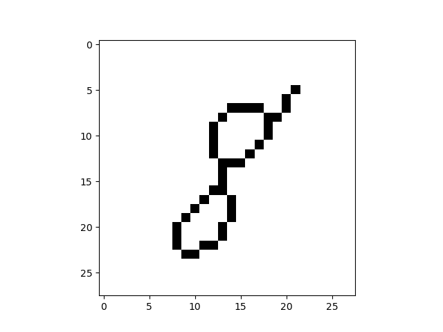
The pre-processing steps to expose the digits topology, shown for the image of a handwritten digit 8 in Figure 3, are the following:
- Load the MNIST image of a handwritten digit.
- Produce a binary image by thresholding.
- Reduce the image to a skeleton of 1-pixel width using the popular Zhang-Suen thinning algorithm.
 |
 |
 |
|---|---|---|
| (1) Original image | (2) Binary image | (3) Skeleton |
To construct the graph $G$ from the 1-pixel width skeleton, we treat the pixels of the skeleton as vertices of $G$ and add the edges between adjacent vertices and then remove all created cycles of length 3. Intuitively, we connect the points while trying not to create new topological features. The result for the image of a handwritten digit 8 is in Figure 4. The resulting graph in this example consists of one connected component with two cycles, so no new topological features were added.

Extracting the topological features
We construct a simplex stream for computing the persistent homology using the following filtration on the graph $G$ embedded in the plane. We are adding the vertices and edges of graph $G$ as we sweep across the plane. From the simplex stream, we compute the persistent homology to get the Betti barcodes. The Dionysus 2 package was used for the computation of persistent homology; see the Source code and package documentation [4] for details.
Figure 5 shows the result of this technique applied on the image of a handwritten digit 8. In this example, we sweep across the plane to the top in a vertical direction $y \in (-\infty, \infty)$.

Betti 0 barcode $\beta_{0}$ consists of one interval $[2, \infty)$, which clearly shows the single connected component with the birth time of 2 when the first vertex of $G$ is added.
Betti 1 barcode $\beta_{1}$ consists of two intervals $[10, \infty)$ and $[18, \infty)$, with birth times of 10 and 18 corresponding to the births of the two cycles. The birth of the cycle is the value of $y$ when the loop closes in the embedded graph $G$ as we sweep to the top.
Finally, we extract the following features from each of the k-dimensional Betti barcodes in the following way. Denote the endpoints of Betti barcode intervals with:
\[x_{1}, y_{1}, ..., x_{n}, y_{n}\]where $x_{i}$ represents the beginning and $y_{i}$ the end of each interval. From the endpoints we compute 4 features from the invariants discussed in [1], that take into account all of the bars lengths, and endpoints:
\[\begin{align*} f_{1}&=\sum_{i} x_{i} (y_{i} - x_{i}) \\ f_{2}&=\sum_{i} (y_{\max} - y_{i})(y_{i} - x_{i}) \\ f_{3}&=\sum_{i} (y_{\max} - y_{i})^{2} (y_{i} - x_{i})^{4} \\ f_{4}&=\sum_{i} x_{i}^{2} (y_{i} - x_{i})^{4} \\ \end{align*}\]For each of the 4 sweep directions: top, bottom, right, left and for each $k$-dimensional Betti barcode, $k = 0, 1$, we compute the defined 4 features $f_{1}, \dots, f_{4}$. This gives us a total of $4 \cdot 2 \cdot 4 = 32$ features per image.
Empirical results
Data set consisted of extracted topological features of 10000 images of handwritten digits from MNIST database. Data set was split 50:50 in train and test set so that each had 5000 examples. SVM with RBF kernel was used for classification of the images based on the extracted topological features. The empirical classification results are as follows. Accuracy on the train set using 10-fold cross-validation was $0.88 (\pm 0.05)$. Accuracy on the test set was 0.89.
We examine the common misclassifications.
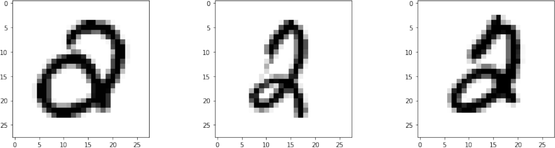
There were 3 examples of the number 2 being mistaken for number 0, shown in Figure 6. The reason is that the number 2 was written with a loop that appears in the region that is close to the loop in number 0.
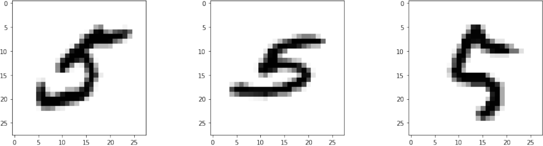
For number 5 we got the lowest F1 score of 0.75. It was misclassified as number 2 in 32 examples in the test set. The first three examples are shown in Figure 7. This was expected since these two numbers are topologically the same with no topological features (e.g. loops) appearing in different regions.
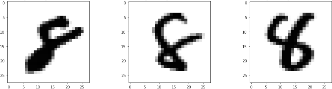
Number 8 was misclassified as number 4 in 21 examples from the test set. The first three examples are shown in Figure 8. We see the stylistic problems that caused the misclassifications. The top loop of number 8 was not closed which made it topologically more similar to number 4 written with a loop.
Source code
The repository containing all Python scripts that I wrote for this tutorial including the processed version of the data set is available in tda-digits repository on GitHub.
It’s dependencies are:
- Python (2 or 3);
- Dionysus 2 for computing persistent homology;
- Boost version 1.55 or higher for Dionysus 2;
- NumPy for loading data and computing;
- Scikit-learn for machine learning algorithms;
- Scikit-image for image pre-processing;
- Matplotlib for plotting;
- Networkx for plotting graphs.
References
[1] A. Adcock, E. Carlsson, and G. Carlsson, “The Ring of Algebraic Functions on Persistence Bar Codes”, (2013), Homology, Homotopy and Applications https://arxiv.org/abs/1304.0530
[2] R. Bruel-Gabrielsson, B. J. Nelson, A. Dwaraknath, P. Skraba, L. J. Guibas, and G. Carlsson, “A Topology Layer for Machine Learning”, (2020), Proceedings of Machine Learning Research https://arxiv.org/pdf/1905.12200.pdf
[3] G. Carlsson, “Topology and data”, (2009), Bulletin of the American Mathematical Society https://www.ams.org/journals/bull/2009-46-02/S0273-0979-09-01249-X/S0273-0979-09-01249-X.pdf
[4] Dmitriy Morozov, “Dionysus 2 documentation”. https://mrzv.org/software/dionysus2/